Object detection like it's the 90s
1. Motivation
1.1 Modern methods
These days object detection is typically done by machinelearning-based methods. The backbone of these methods are Convolutional Neural Networks (CNNs). Such methods are typically divided in one-stage and multiple-stage ones and some popular ones are YOLO, SSD and faster RCNN and its derivatives. Let’s look at them briefly to show how fundamentally differenly they are to the classical method that I will present.
| Name | Stages | Description |
|---|---|---|
| YOLO | One | Divide an image in a grid. For each cell, describe it with (1) a class probability and (2) some bounding boxes with height, width, centre and confidence. Then, non-max suppression to compute the Intersection of Union (IoU) and reject overlapping boxes and keep only the one with highest confidence. |
| SSD | One | Assigns class probabilities similarly to YOLO. The difference is that it performs detection at multiple resolutions and produces bounding boxes of fixed size (anchors) at each. Sums the multi-res maps and compares the IoU to a threshold to derive final bounding boxes. |
| faster RCNN | Many | Selective search to draw boxes around object candidates. Warp each region around a fixed size and pass it to a CNN which computes features. Feed features to a classifier. Non- max suppression to eliminate redundant boxes. |
These are pretty accurate and work in real time. However, they require high computational power. A lot of modern approaches struggle to run in real-time without CPUs specialised in AI. Getting them to run can also be a pain because of all the libraries they require (and trust me, I’ve been through that pain a lot). This makes them unsuitable for low-power devices.
1.2 The idea of matching via histograms
This is where a very elegant and lightweight approach from the 90s by M. Swain and D. Ballard comes in handy, and that is histogram backprojection. As the name suggests, this relies on colour operations (histogram) as opposed to point operations (pixel locations). It cannot do full object detection on its own, but it’s very good at matching two images.
2. Histogram backprojection
2.1 Input/Output
The input is an RGB image $I_{m \times n}$ and a model $M$. The histogram of the model describes what we want to match at every region of the image $I$. The algorithm outputs an image $b_{m\times n} \in [0,1]$.
The closer each value of $b$ to 1, the better the match.
2.2 Histogram ratio
The backprojection method relies on the histogram ratio as a matching criterion between two images to let’s define it as $R$:
$R = \frac{H_M}{H_I}$
, where $H_M, H_I$ are the histograms of the model and image respectively.
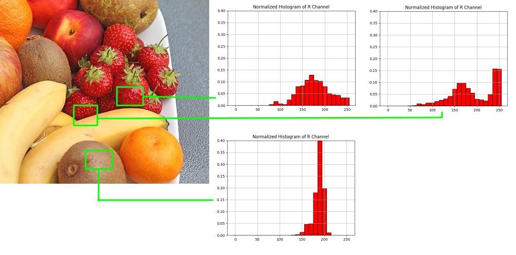
To demonstrate what the ratio means for the two images, we will only consider the histogram of the red channel. Therefore $H_M$, $H_I$ are 255-length vectors. We will also normalise them. In general, however, $H_M$ and $H_I$ are 2D matrices and they never measure just one channel. We will try to understand what the values of $R$ mean.
Let’s look at the picture of fruit below, use the pure strawberry as a model and match it with two samples of the image. When computing the histograms, we isolate the R channel of the RBG and obviously the two strawberry histograms look similar. The idea is that the model contains high values in some narrow band. Therefore for the colour tones at the range that describes the model, it will be true that $H_{M_i} > H_{I_i}, \; i \in [0, 255]$ or $R_i = \frac{H_{M_i}}{H_{I_i}} > 1$. In the picture below, histogram intensities are binned every 5, hence the bar charts.
Now if we look at the ratio histograms between the model and the half-strawberry half-banana sample (good match), we observe a peak at the range that describes the model. If we also look at a bad match, for example the strawberry and the skin of a kiwi, it’s mostly zero.
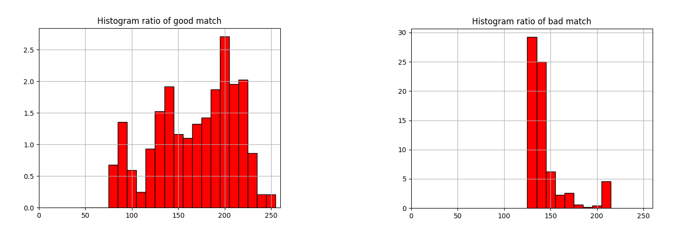
Therefore every characteristic colour tone $i$ of the model has a high ratio ${M_i}/H_{I_i}$.
2.3 Colour spaces
Before the algorithm is introduced, it is important to know that the histogram is never computed from an RGB image. RBG colour space is susceptible to illumination changes therefore the same object can have two different RGB histograms in two different illumination conditions. Colour spaces such as HSV or sRBG are preferred because they mitigate this. In this case I’ll be using HSV. Its components are:
- H (Hue): the perceived colour
- S (Saturation): How vivid a colour appears relative to its
- V (value): The brightness
Unlike RGB, which a cubic colour coordinate system, HSB is a cylindrical one where hue is described by an angle from 0 to 360 degrees, saturation as the radius and value as the height.

Hue and saturation don’t change under illumination, that’s why HSV is a good space to filter an object’s colours. The conversion from RGB to HSV involves several steps and the equations are presented here.
2.4 The Histogram Backprojection Algorithm
The main idea of the algorithm is that every colour is replaced by its histogram ratio. In other words, we project the histogram ratio back into the original image.
Let $I$ be the image where we’re looking to match the object and $M$ a smaller model image whose histogram describes what we’re looking to match.
First, let’s define a function that given two images of the same size, it computes a single backprojection value.
Compute a single backprojection value
Inputs: $I_{m\times n}$, $M_{m\times n}$, some indices $0 \leq i \leq m$, $0 \leq j \leq n$
Output: a scalar from 0 to 1function $backproject(I, M, i, j)$:
$\quad$ $H_I \leftarrow histogram(I)$
$\quad$ $H_M \leftarrow histogram(M)$
$\quad$ for each histogram bin $i$:
$\qquad$ $R_i \leftarrow \min(\frac{H_M}{H_I}, 1)$
$\quad$ $color \leftarrow I_{ij}$
$\quad$ return $R_{color}$
We clip $R$ to 1: $R_i \leftarrow \min(\frac{H_M}{H_I}, 1)$ as values more than one would skew the distribution. Now if $I$ is a large image, we slide $M$ over it and compute the backprojection for each pixl of $I$. Furthermore $b$ is convolved with a disc to smoothen the predictions.
Compute backprojection image
Inputs: $I_{m\times n}$, $M_{a\times b}$
Output: $b_{m\times n}$function $backprojection(I, M)$:
$\quad$ $b \leftarrow zeros(m, n)$
$\quad$ for $i$ in $0..m$:
$\qquad$ for $j$ in $0..n$:
$\qquad$ $\quad$ $b_{ij} \leftarrow$ backproject($I, M, i, j$)
$\quad$ $b \leftarrow b * D_r$
$\quad$ return $b$
$*$ denotes convolution and $D_r$ is a disc of radius $r$, so it’s defined as:
\(D_r =\)
To localise the object and as the authors suggest, we can find the indices of $\max(b)$.
The next step is optional and it can be scaling the image from 0 to 255 and applying thresholding it - setting high values to 255 and low ones to 0. Otsu’s is an automatic thresholding method tha1t can be used.
2.5 (Optional) Conversion to black and white - Otsu’s method derivation
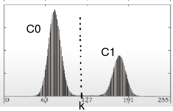
Otsu’s method assumes a gray scale image is bimodal - i.e. consists of two classes; $C_0$ and $C_1$ (background and foreground or vice versa). Visually such a distribution looks like two lobes. We also assume that the distribution is normalised. Otsu’s method seeks the best threshold $k$ to separate $C_0$ and $C_1$.
What do “classes” mean in this case? $C_0$ and $C_1$ are not known in advance, they’re non-overlapping and each is described by two intensity indices. Otsu aims to separate them based on an intensity $k$ - the upper bound of $C_0$ and lower bound of $C_1$.
After this is done, any histogram intensity $i<k$ gets mapped to $0$ and everything else gets mapped to $255$.
If the image is represented by $L$ levels (e.g. $L=256$ for an 8-bit image), then each probability $p_i$ in the histogram represents the probability that a random pixel will have the value $i$ and it’s true that
$ \sum\limits_{i=0}^{L-1} p_i = 1 $
Now suppose we dischotomise the pixels in two classes $C_0$ and $C_1$ for some arbitrary threshold $k \in [0, L-1]$. So pixels in $C_0$ range from 0 to $k-1$ and pixels in $C_1$ from $k$ to $L-1$. The total probabilities (or number of observations) of each class as a function of $k$ are:
$\omega_0 = Pr(C_0) = \sum\limits_{i=0}^{k-1} p_i = \omega(k)$
$\omega_1 = Pr(C_1) = \sum\limits_{i=k}^{L-1} p_i = 1 - \omega(k)$
The goal is to express the variance of each class in terms of $k$ so we calculate their means first. Each class is treated independently when calculating its means so the conditional probability is used.
$\mu_0 = \sum\limits_{i=0}^{k-1} i \, Pr(i|C_0)$
However, from Bayes rule:
$Pr(i|C_0) = \frac{Pr(C_0|i) Pr(i)}{Pr(C_0)} = \frac{1\cdot i}{\omega_0}$
($Pr(C_0|i)=1$ holds because $0 \leq i \leq k-1$, so $i$ belongs in class 0)
Therefore for $\mu_0$:
$\mu_0 = \sum\limits_{i=0}^{k-1} \frac{ip_i}{\omega_0} = \frac{\mu(k)}{\omega_0}$
where $\mu(k)$ is the mean up to level $k-1$ (aka first-order moment):
$\mu(k) = \sum\limits_{i=0}^{k-1}ip_i$
Similarly, for the mean of class $C_1$ we can write:
$\mu_1 = \sum\limits_{i=k}^{L-1} \frac{ip_i}{\omega_1}$
However, $\sum\limits_{i=k}^{L-1} ip_i = \sum\limits_{i=0}^{L-1}ip_i - \sum\limits_{i=0}^{k-1}ip_i = \mu_{tot} - \mu_0$ and $\omega_1 = 1 - \omega_0$. Therefore $\mu_1$ is written as:
$\mu_1 = \frac{\mu_{tot} - \mu_0}{1-\omega_0}$
Therefore it’s easy to verify that:
$\mu_0\omega_0 + \mu_1\omega_1 = \mu_{tot}$
Now we can begin computing the variance for each class. Each conditional probability can be expanded by Bayes rule just like it was done earlier.
$\sigma_0^2 = \sum\limits_{i=0}^{k-1} (i-\mu_0)^2 Pr(i|C_0) = \sum\limits_{i=0}^{k-1} (i-\mu_0)^2 p_i/\omega_0$
$\sigma_1^2 = \sum\limits_{i=k}^{L-1} (i-\mu_1)^2 Pr(i|C_1) = \sum\limits_{i=k}^{L-1} (i-\mu_1)^2 p_i/\omega_1$
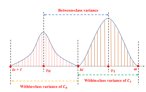
The within-class variance $\sigma_{within}^2$ measures how spread out each class is. It’s defined as the sum of the two class variances multiplied by their associated weight.
$\sigma_{within}^2 = \omega_0\sigma_0^2 + \omega_1\sigma_1^2$
$ \qquad \quad = \omega_0\sum\limits_{i=0}^{k-1}(i-\mu_0)p_i/\omega_0 + \omega_1\sum\limits_{i=k}^{L-1}(i-\mu_1)p_i/\omega_1$
$ \qquad \quad = \sum\limits_{i=0}^{k-1}(i-\mu_0)p_i + \sum\limits_{i=k}^{L-1}(i-\mu_1)p_i$
We also compute the total “between-class” variance, which measures how far away the lobes are. We compute the total between class variation for each class as the difference between the class mean and the grand mean multiplied by the number of observations in each class:
$\sigma_{between}^2 = \omega_0(\mu_{tot} - \mu_0)^2 + \omega_1(\mu_{tot} - \mu_1)^2 = \ldots = \omega_0\omega_1(\mu_1-\mu_0)^2$
To maximimise the separability between $C_0$ and $C_1$ and therefore find the optimal thrshold, we want to minimise the within-class class variance and maximise the between-class variance $\sigma^2_{between}$. However, with a bit of algebra we will show that
$\sigma_{between}^2 + \sigma_{within}^2 = \sigma_{tot}^2 = const$
, where $\sigma_{tot}^2$ is constant and equal to the total variance of the image. Therefore the minimisation and maximisation are equivalent. To prove the latter equation begin with $\sigma_{tot}^2$.
$\sigma_{tot}^2 = \sum\limits_{i=0}^{L-1} (i-\mu_{tot})^2 p_i$
$\qquad = \underbrace{\sum\limits_{i=0}^{k-1} (i-\mu_{tot})^2 p_i}_{A} + \underbrace{\sum\limits_{i=k}^{L-1} (i-\mu_{tot})^2 p_i}_{B}$
$A = \sum\limits_{i=0}^{k-1} (i-\mu_0 + \mu_0 - \mu_{tot})^2 p_i = \sum\limits_{i=0}^{k-1}p_i \Big((i-\mu_0)^2 + 2(i-\mu_0)(\mu_0-\mu_{tot}) + (\mu_0 - \mu_{tot})^2\Big)$
$B = \sum\limits_{i=k}^{L-1} (i-\mu_1 + \mu_1 - \mu_{tot})^2 p_i = \sum\limits_{i=k}^{L-1}p_i \Big((i-\mu_1)^2 + 2(i-\mu_1)(\mu_1-\mu_{tot}) + (\mu_1 - \mu_{tot})^2\Big)$
Therefore $\sigma_{tot}^2$ is expanded as
$\sigma_{tot}^2 = \sum\limits_{i=0}^{k-1}p_i \Big((i-\mu_0)^2 + 2(i-\mu_0)(\mu_0-\mu_{tot}) + (\mu_0 - \mu_{tot})^2\Big) +$ $\qquad \quad \sum\limits_{i=k}^{L-1}p_i \Big((i-\mu_1)^2 + 2(i-\mu_1)(\mu_1-\mu_{tot}) + (\mu_1 - \mu_{tot})^2\Big)$
Now examine each term.
- first squared terms: $\sum\limits_{i=0}^{k-1}p_i (i-\mu_0)^2 + \sum\limits_{i=k}^{L-1}p_i (i-\mu_1)^2 = \omega_0\sigma_0^2 + \omega_1\sigma_1^2 = \sigma_{within}^2$
- cross-product terms: $\sum\limits_{i=0}^{k-1} (i-\mu_0)p_i = 0$ - see the definition of $\mu_0$ $\therefore \; \sum \limits_{i=0}^{k-1} p_i(i-\mu_0)(\mu_0-\mu_{tot}) = \sum \limits_{i=k-1}^{L-1}p_i(i-\mu_1)(\mu_1-\mu_{tot}) = 0$
- last squared terms: $\sum\limits_{i=0}^{k-1}p_i (\mu_0 - \mu_{tot})^2 + \sum\limits_{i=k}^{L-1}p_i(\mu_1 - \mu_{tot})^2 =$ $(\mu_0 - \mu_{tot})^2\sum\limits_{i=0}^{k-1}p_i + (\mu_1 - \mu_{tot})^2\sum\limits_{i=k}^{L-1}p_i = (\mu_0 - \mu_{tot})^2\omega_0 + (\mu_1 - \mu_{tot})^2\omega_1 = \sigma_{between}^2$
$\therefore \; \sigma_{tot}^2 = \sigma_{within}^2 + \sigma_{between}^2$
So in the end the objective is to find $k := \text{argmax}(\omega_0\omega_1 (\mu_1 - \mu_0)^2)$. This is achieved with a simple iterative search therefore the time complexity of Otsu is $\mathcal{O}(LN)$, where $N$ is the number of pixels.
Because of that, the maximisatoin can easily be implemented in just one line of Python. However I will break it down for readability:
def otsu(histogram) -> int:
    """
    Input: 1D normalised histogram
    Return: some threshold k with 0 < k < 255
    """
    return np.argmax([
        np.sum(histogram[:k]) * (1 - np.sum(histogram[:k])) *
        (
             np.sum([i * pi for i, pi in enumerate(histogram[:k])]) / np.sum(histogram[:k]) -
             np.sum([(k + i) * pi for i, pi in enumerate(histogram[k:])]) / np.sum(histogram[k:])
        )**2 if np.sum(histogram[:k]) > 0 and np.sum(histogram[k:]) > 0 else 0
        for k in range(256)
    ])
In the original paper, Otsu treats the case of multiple equal peaks but I’ll skip this. Apart from that case, the implementation outputs the same threshold as OpenCV would. Let’s see an output.
import cv2
import numpy as np

np.random.seed(1337)
image = np.random.randint(0, 256, (14, 14), dtype=np.uint8)
histogram = cv2.calcHist([image], [0], None, [256], [0, 256])
histogram /= np.sum(histogram)
thresh = otsu(histogram)
image[image < thresh] = 0
image[image >= thresh] = 255
2.6 Implementing Backprojection with Otsu for Object Detection
To reiterate, we are given an image $I$ and a sample $M$ of the object to match. The goal is to obtain a new “backprojected” image where the matched object pixels remain the same and everything else is black. The steps are:
- Convert $I$, $M$ from RGB to HSV or another domain.
- Compute the ratio histogram.
- Replace every colour in the original image with its value on the ratio histogram.
- Convolce the latter backprojected image with a disc.
- Scale the values from 0 to 255 and apply Otsu’s threshold to find a white mask.
- bitwise AND the mask with the original image $I$.
All that is implemented below using OpenCV’s functions to compute the histogram, Otsu’s threshold
and convolution. The histogram is 2D - the HS of HSV for each image.
Not also that the histogram is not divided as $[0,1],[1,2]\ldots,[254,255]$, but it’s binned,
e.g. as $[0,5], [5,10],\ldots,[250,255]$. When using the program, the user is shown an image
where the object is shown and one or more samples of the object can be selected by drawing one or more
rectangles and then pressing c via the crop_with_mouse function. Then it will perform matching
via backprojection and show the matched result as non-black. To stay true to the authors’ rationale
that backprojection is also used for localisation, the backproject function returns the black and white
image (mask) and the location (pixel) of the maximum backprojected value. This location can be plotted
by uncommenting line #cv2.circle(result_image, (locmax[1], locmax[0]), 3, (255, 50, 0), 4). However it’s
not helpful for the big objects I’ll be matching.
import cv2
import numpy as np
from typing import List, Tuple


def hsv_histogram(image, h_bins=50, s_bins=60, convert_to_hsv=True):
    if convert_to_hsv:
        hsv_image = cv2.cvtColor(image, cv2.COLOR_BGR2HSV)
    return cv2.calcHist([hsv_image], [0, 1], None, [h_bins, s_bins], [0, 180, 0, 256])

def create_circular_mask(rad):
    diam = 2*rad
    mask = np.zeros((diam, diam), dtype=np.float32)
    y, x = np.ogrid[0:diam, 0:diam]
    mask[(x-rad)**2 + (y-rad)**2 <= rad**2] = 1
    # it's important that the mask is normalised otherwise convolution leaks values!
    mask /= np.sum(mask)
    return mask

def backproject_multiple(image, models: List[np.ndarray], h_bins=50, s_bins=60):
    backprojection = np.zeros((image.shape[0], image.shape[1]), dtype=np.float32)
    image_hist = hsv_histogram(image)
    model_hist = np.zeros((h_bins, s_bins), np.float32)
    rad = 0
    for model in models:
        model_hist += hsv_histogram(model)
        rad += min(model.shape[:2])/2
    rad = int(rad/len(models))
    model_hist /= len(models)
    ratio_hist = np.divide(model_hist, np.where(image_hist == 0, 1, image_hist))
    hsv_image = cv2.cvtColor(image, cv2.COLOR_BGR2HSV)
    for i in range(image.shape[0]):
        for j in range(image.shape[1]):
            h_bin_size, s_bin_size = 180/h_bins, 256/s_bins
            h_val, s_val = int(hsv_image[i, j, 0] / h_bin_size), int(hsv_image[i, j, 1] / s_bin_size)
            backprojection[i, j] = min(ratio_hist[h_val, s_val], 1)
    # most likely location of object
    ind_max = np.argmax(backprojection)
    loc_max = np.unravel_index(ind_max, backprojection.shape)

    ### Post-processing
    # normalize backprojection to the range [0, 255]
    backprojection = cv2.normalize(backprojection, None, 0, 255, cv2.NORM_MINMAX)
    #rad = min(model.shape[0], model.shape[1]) // 2
    circular_mask = create_circular_mask(rad)
    # convolve with circular mask to spread the values around
    backprojection = cv2.filter2D(backprojection, -1, circular_mask).astype(np.uint8)
    # Apply Otsu's threshold to keep highe values only
    _, backprojection = cv2.threshold(backprojection, 0, 255, cv2.THRESH_BINARY | cv2.THRESH_OTSU)
    return backprojection.astype(np.uint8), loc_max


def backproject(image, model, h_bins=50, s_bins=60) -> Tuple:
    backprojection = np.zeros((image.shape[0], image.shape[1]), dtype=np.float32)
    image_hist = hsv_histogram(image)
    model_hist = hsv_histogram(model)
    ratio_hist = np.divide(model_hist, np.where(image_hist == 0, 1, image_hist))

    ### b[x,y] = R[Ihsv[x,y]]
    hsv_image = cv2.cvtColor(image, cv2.COLOR_BGR2HSV)
    for i in range(image.shape[0]):
        for j in range(image.shape[1]):
            h_bin_size, s_bin_size = 180/h_bins, 256/s_bins
            h_val, s_val = int(hsv_image[i, j, 0] / h_bin_size), int(hsv_image[i, j, 1] / s_bin_size)
            backprojection[i, j] = min(ratio_hist[h_val, s_val], 1)
    # most likely location of object
    ind_max = np.argmax(backprojection)
    loc_max = np.unravel_index(ind_max, backprojection.shape)

    ### Post-processing
    # normalize backprojection to the range [0, 255]
    backprojection = cv2.normalize(backprojection, None, 0, 255, cv2.NORM_MINMAX)
    rad = min(model.shape[0], model.shape[1]) // 2
    circular_mask = create_circular_mask(rad)
    # convolve with circular mask to spread the values around
    backprojection = cv2.filter2D(backprojection, -1, circular_mask).astype(np.uint8)
    # Apply Otsu's threshold60 to keep highest values
    _, backprojection = cv2.threshold(backprojection, 0, 255, cv2.THRESH_BINARY | cv2.THRESH_OTSU)
    return backprojection.astype(np.uint8), loc_max

def apply_mask(image, backprojection):
    return cv2.bitwise_and(image, image, mask=backprojection)


def crop_with_mouse(image_path):
    # global variables
    ref_point = []
    cropping = False
    cropped_images = []

    def click_and_crop(event, x, y, flags, param):
        nonlocal ref_point, cropping
        # hold left click to start drawoing
        if event == cv2.EVENT_LBUTTONDOWN:
            ref_point = [(x, y)]
            cropping = True
        # release left click to stop drawing
        elif event == cv2.EVENT_LBUTTONUP:
            ref_point.append((x, y))
            cropping = False
            # draw a rectangle around the region of interest
            cv2.rectangle(image, ref_point[0], ref_point[1], (0, 255, 0), 2)
            cv2.imshow("select area and then press c", image)
            # crop the region of interest and store it
            if len(ref_point) == 2:
                x0, y0 = ref_point[0]
                x1, y1 = ref_point[1]
                roi = clone[min(y0, y1):max(y0, y1), min(x0, x1):max(x0, x1)]
                cropped_images.append(roi)
                ref_point = []  # Reset ref_point for next cropping
    # load the image, clone it, and setup the mouse callback function
    image = cv2.imread(image_path)
    clone = image.copy()
    cv2.namedWindow("select area and then press c")
    cv2.setMouseCallback("select area and then press c", click_and_crop)

    while True:
        # display the image and wait for a keypress
        cv2.imshow("select area and then press c", image)
        key = cv2.waitKey(1) & 0xFF
        # if 'r' is pressed, reset the cropping region
        if key == ord("r"):
            image = clone.copy()
        # if 'c' is pressed, break from the loop
        elif key == ord("c"):
            break
    cv2.imwrite('input.png', image)
    cv2.destroyAllWindows()
    return cropped_images


if __name__ == '__main__':
    impath = 'orchids.png'
    im = cv2.imread(impath)
    models = crop_with_mouse(impath)
    if len(models) == 1:
        model = models[0]
        backprojection, locmax = backproject(im, model)
        result_image = apply_mask(im, backprojection)
        #cv2.circle(result_image, (locmax[1], locmax[0]), 3, (255, 50, 0), 4)
    else:
        backprojection, _ = backproject_multiple(im, models)
        result_image = apply_mask(im, backprojection)
    cv2.imwrite('output.png', result_image)
    cv2.imshow('Backprojection', result_image)
    cv2.waitKey(10000)
    cv2.destroyAllWindows()
| Input & drawn sample(s) | Output |
|---|---|
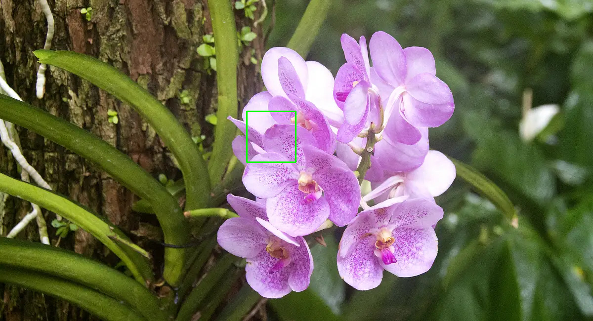 |
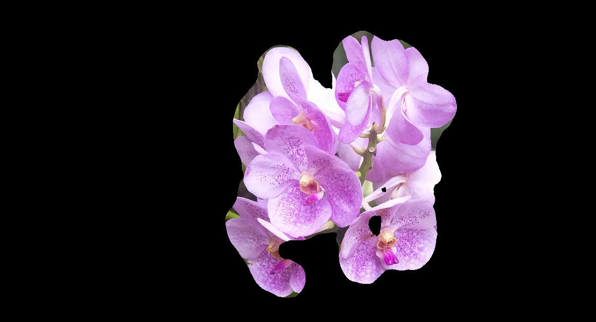 |
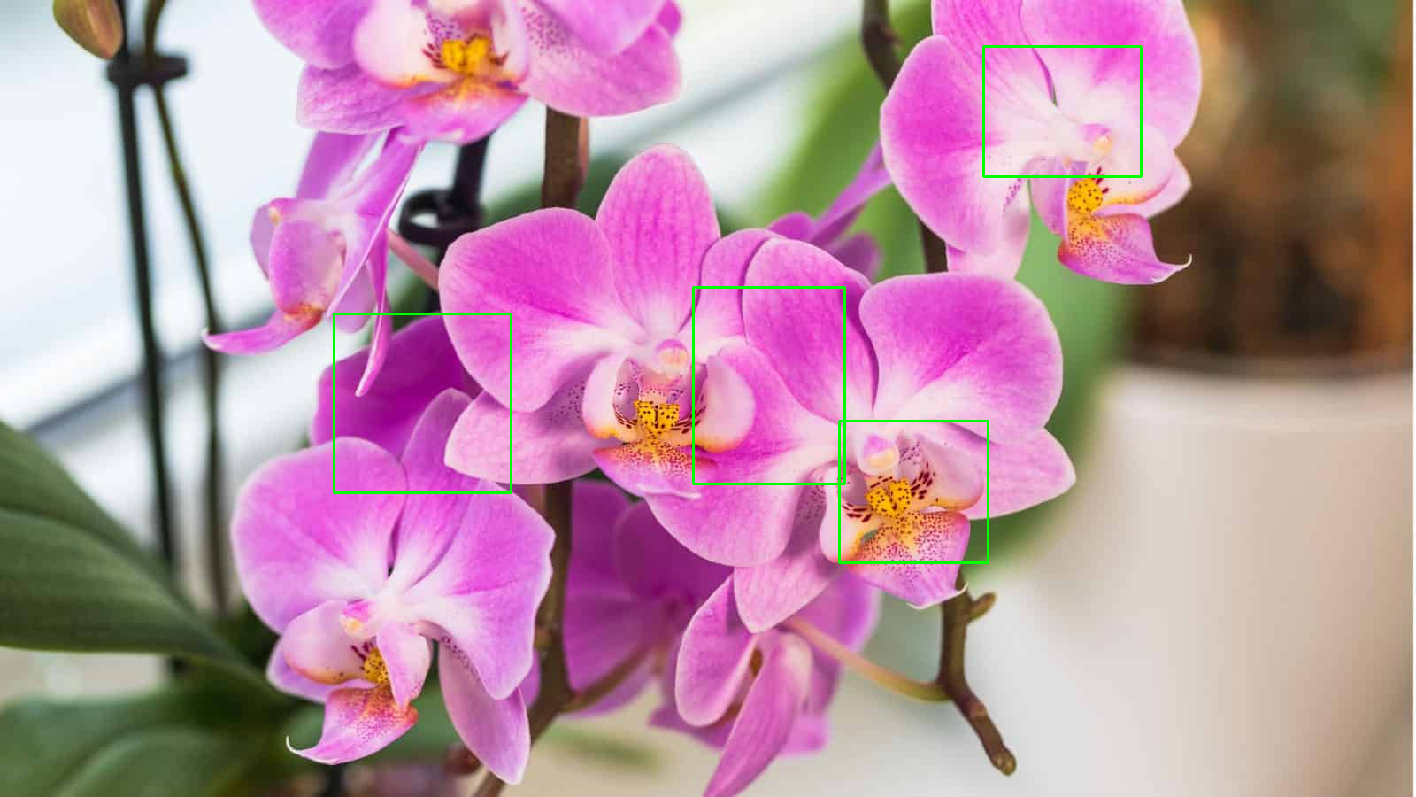 |
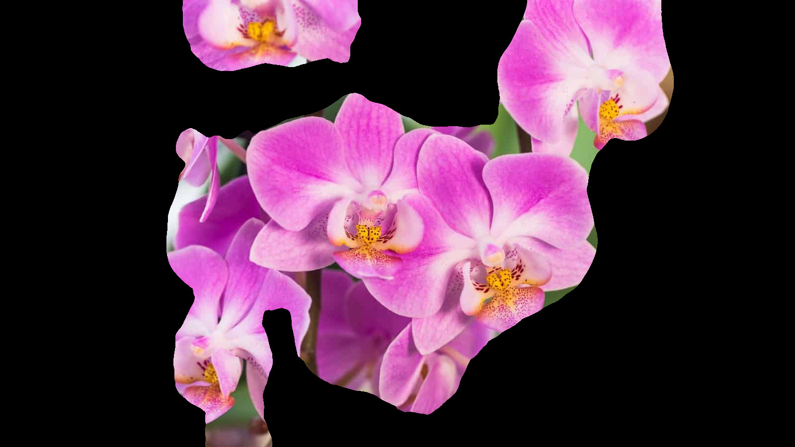 |
Not bad for such a simple algorithm when matching those orchids, right?
3. Closing thoughts
Histogram backprojection is used for object matching given a small sample of the object. It only relies on colour and completely ignores spatial information. Remember to always convert the input image to a domain that’s not susceiptible to illumiation changes before running the algorith, such as HSV. The algorithm uses 2D histograms, such as across HS. It may not be as good as flow-based segmentation methods or modern semantic segmentation but it’s way simpler to implement and with some optimisations it can work in real time. To improve the algortihm’s accuracy, one can stitch together various samples of the same object int a supersample (e.g. skin from different humans) and use this.
In this article it was used for object detection – not recognition. There are a couple of ways the algorithm can be adapted for recognition. One way is by keeping a database of models from various objects, performing backprojection with each model $M$, and summing all the values in the backprojected image. The sum with the highest value corresponds to the best recognised object. However, for simple recognition we don’t even need the backprojection. Again, given a database of models, we can compute the histogram $H(M)$ of each and the histogram of the input image $H(I)$. The model with the best match corresponds to the object contained in the input image $I$. This method is also described in Swain’s paper and the histogram intersection function used there is:
$int(H(I), H(M) = \frac{\sum\limits_{i=0}^n \min\big(H(I)_i, H(M)_i\big)}{\sum\limits_{i=0}^n H(M)_i}$
, where $n$ is the number of bins and $i$ each bin. Obviously intersection ranges from 0 to 1. This expression may look complicated but if we can scale (downsample) the image histogram to be the same size as the model histogram and then re-normalise it, i.e. if
$\sum\limits_{i=0}^n H(I)_i = \sum\limits_{i=0}^n H(M)_i$
then this intersection expression is simplified to:
$1 - int(H(I), H(M)) = \frac{1}{N}\sum\limits_{i=0}^n \left|H(I)_i - H(M)_i \right|$
Why is either of these a good measure of intersection? Make up some good and bad-matching histograms, draw them and estimate how close the intersection is to 0 or 1.
On another note, it may come as a surprise but backprojection is not only good for object matching! It can be used as a feature extractor for mean shift or other methods to build trackers. They work together surprisingly well and in real time. But that’s all for now.