Building a Head and Hand Recognition System with Kinect
0. Goals
Body part recognition is the cornerstone of most AR applicatoins, with the head and hand being particularly valuable. Microsoft Kinect facilitates this by capturing RGB and depth (RGBd) images. Not only that, but it’s also suitable for the development of AR desktop applications without the need of a GPU.
In this article, I will show you how to build a head and hand detection system from scratch, which can be broken down to the following goals:
- Interface with a Kinect (on Linux) and capture some data.
- Learn some underlying concepts about Kinect’s functionality.
- Learn the key parts of the theory required for body part classification from depth images.
- Lean how to train a body part classifier from depth image data.
- Put everything together in a system that draws bounding boxes around the hands and head.
Why? Yes, Microsoft provides a Kinect SDK with Linux support. The SDK detects the landmarks of each body part. However not all cameras come equipped with a SDK. Plus, if we can develop a body part classifier for Kinect, the same method can be generalised for any depth camera.
This article is meant to be accompanied by my kinect-rf repository, which includes the practical implementation.
1. Kinect’s Components
1.1. Brief History
Microsoft Kinect is a discontinued motion sensor device. It used to be an Xbox addon and during its development (circa 2005 to 2014) motion sensor peripherals were all the rage in consoles. It comes in two versions - v1 and v2 and it’s able to capture RGB depth (RGBd) frames.
1.2. Ways to Measure Depth
Kinect v1 uses light coding (LC) to measure the relative distance of objects. It emits an infrared pattern of light (e.g. spaced stripes) and by inspecting the wrapping and thickness of the received lines, geometric information about the object is derived. It’s reliable but requires calibration. The main disadvanage of LC is that it’s affected by ambient light and it’s susceptible to imperfections of the reflected object’s texture.
On the other hand, Kinect v2 uses a time-of-flight (ToF) camera. ToF relies on emitting modulating sine waves and measuring the phase difference between the emitted and received wave, which allows to measure the travel time. It requires high-precision hardware which however is typically small. It has a wider field of view than light coding and does not require any algorithm to decode the geometry. However it consumes more power than LC.
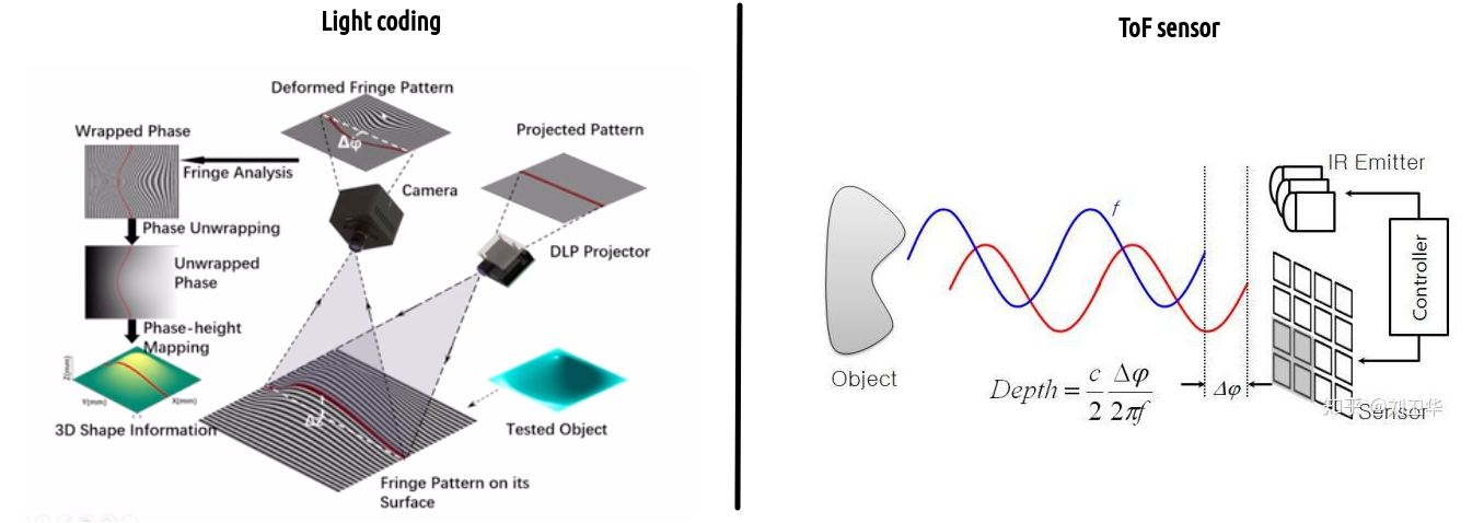 Fig. 1. Operation of LC vs ToF [1] [2].
1.3. Main Components
Kinect is equiped with a single RGB camera, an infrared (IR) emitter, an IR receiver and some other components that are not relevant in this article.

Fig. 2. Operation of LC vs ToF [3].
Before we get into the setup, I present how ToF sensors measure distances as ToF is more widespread technology.
2. Basics of ToF cameras
2.1. Hardwave components
A ToF camera works by illuminating the scene with modulated waves via a laser or LED. The emitted wave $e(t)$ is typicallly of short infrared wavelength (~700-1000 nm). The wave is emitted via a grid-line arrnagement of Near Infrared (NIR) emitters. The arrangement simulates a point source so the wave can effectively be considered to be emitted from its centre.
As you can see, emitters are distributed around the lock-in pixels matrix and mimic a simulated emitter co-positioned with the center of the lock-in pixel matrix.

Fig. 3. A Near InfraRed (NIR) emitter [4].
The receiver is typically some photo diode arrangement coupled with a low-pass filter, followed by a correlation hardware (typically a multiplier circuit).
The next important design decision is the emitted light’s waveform. The waveform can be constructed either with Direct Pulse Modulation (DPM) - which results in a rectangular wave or Direct Continuous Wave Modulation (DCWM), which results in a sinusoid. The more common way is DPM, however we’ll discuss DCWM as it has broader applications outside of ToF cameras.
2.2. Determining DCWM’s modulation parameters
The emitted wave of modulation frequency $f_m$ is described by (amplitude of $1$ for reference):
$e(t) = \cos(2\pi f_m t) = \cos(\omega_m t)$
The distance between the laser emitter and the reflected object can easily be recovered from the emitted wave’s phase shift $\Delta \phi, \, 0 \leq \Delta \phi \leq 2 \pi$ during the round-trip:
$d = \frac{c}{4\pi f_m} \Delta \phi$
The received signal after the reflection is:
$r(t) = B + A \cos(\omega_m t - \Delta \phi)$
- $A$ is the amplitude of the received signal and it depends on the object’s reflectivity and of the sensor’s sensitivity. It tends to decreases with $1/d^2$ mainly due to light spreading, i.e. $A \tilde{} 1/d^2$.
- $B$ is an offset coefficient due to the ambient illumination.
What the photo diode sensor can measure it the cross-correlation between the emitted and received signal, which measures how similar $e(t)$ and $r(t)$ are at some time delay $\tau$. The cross correlation is defined as:
$c(\tau) = r * e := \frac{1}{T}\int_{-\infty}^{\infty} r(t) e(t - \tau) \ dt$
It’s impractical to compute this over an infinite time window so instead we compute it over a finite large enough time window of width $T$ ($T$ has nothing to do with period so don’t confuse them). Then the latter integral is rewritten as:
\(c(\tau) = \int_{-\infty}^{\infty} r(t) e(t - \tau) dt = \lim_\limits{T\to\infty} \int_{-T/2}^{T/2} \Big(B + A \cos(\omega_m t - \Delta \phi) \Big) \cos(\omega_m t - \omega_m \tau) \ dt\) \(\qquad = \lim_\limits{T\to\infty} \underbrace{\int_{-T/2}^{T/2} B \cos(\omega_m t - \omega_m \tau)\ dt}_{I} + \lim_\limits{T\to\infty} \underbrace{\int_{-T/2}^{T/2} A\cos(\omega_m t - \Delta \phi) \cos(\omega_m t - \omega_m \tau) \ dt}_{J}\)
For $I$, by changing variables so that $u:= \omega_m t - \omega_m \tau$, $dt = \frac{du}{\omega_m}$, it’s rewritten as:
$ I = \frac{B}{T} \frac{1}{\omega_m} \int_{-\pi - \omega_m}^{\pi - \omega_m} \cos(u)\ du $
$I$ is a bit tricky. In theory, it is possible to integrate precisely over a full period; in that case it would be $0$. However in reality because of slow shutter speed at the receiver end or imperfect sampling, $I$ is not zero and it’s equal to $cB$. We will consider the real-life scenario and let $I = B’$, where $B’ := cB$.
For $J$, we make use of the identity:
$ \cos(\alpha) \cos(\beta) = \frac{\cos(\alpha-\beta) + \cos(\alpha+\beta)}{2} $
Then:
$J = \frac{A}{2T} \int\limits_{-T/2}^{T/2} \Big( \cos((\omega_m t - \Delta \phi)- (\omega t - \omega \tau)) + \cos((\omega_m t - \Delta \phi) + (\omega_m t - \omega_m \tau))\Big) \ dt$ \(\quad \; = \frac{A}{2T} \underbrace{ \int\limits_{-T/2}^{T/2} \cos(\omega_m \tau - \Delta \phi) \ dt}_{K} + \frac{A}{2T} \underbrace{\int\limits_{-T/2}^{T/2} \cos(\omega_m t - \Delta \phi - \omega_m \tau) \ dt}_{L}\)
$ K = \cos(\omega_m \tau - \Delta \phi) \int\limits_{-T/2}^{T/2} \ dt = T\cos(\omega_m \tau - \Delta \phi) $
It’s trivial to see that $L = 0$.
In the end, what we are left with for $c(\tau)$ is:
$c(\tau) = B’ + \frac{A}{2T} K = B’ + \frac{A}{2}\cos(\omega_m \tau - \Delta \phi)$
There are three unknowns to be detmined; $A$, $B’$ and $\Delta \phi$. These can now be determined using the receiving sensor’s measurements. The sensor can keep track of the delay $\tau$ and it can read $c(\tau)$ values. Therefore at least 3 measurements are required, however ToF cameras use a neat interferometry method called 4-bucket method which of course employs 4 measurements.

Fig. 4.The 4-bucket method [5].
This method takes 4 measurements (‘‘buckets’’) of $c(\tau)$ conveniently at delays $\tau_1,\ \tau_2,\ \tau_3,\ \tau_4$ such that:
- $\omega_m \tau_1 = 0$, with $c(\tau_1) = B’ + \frac{A}{2}\cos(\Delta \phi)$
- $\omega_m \tau_2 = \pi/2$, with $c(\tau_2) = B’ + \frac{A}{2}\cos(\frac{\pi}{2} - \Delta\phi) = B’ + \frac{A}{2}\sin(\Delta \phi)$
- $\omega_m \tau_3 = \pi$, with $c(\tau_3) = B’ + \frac{A}{2}\cos(\pi - \Delta\phi) = B’ - \frac{A}{2}\cos(\Delta \phi)$
- $\omega_m \tau_4 = 3\pi/2$, with $c(\tau_4) = B’ + \frac{A}{2}\cos(\frac{3\pi}{2}- \Delta\phi) = B’ - \frac{A}{2}\sin(\Delta \phi)$
From these 4 measurements, it’s straighforward to extract the following:
- amplitude: $A = \sqrt{\left(c(\tau_1) - c(\tau_3)\right)^2 + \left(c(\tau_2) - c(\tau_4)\right)^2}$
- phase shift: $\Delta \phi = \arctan\left(\frac{c(\tau_2)}{c(\tau_1)} \right)$
- ambience constant: $B’ = \frac{c(\tau_1) + c(\tau_2) + c(\tau_3) + c(\tau_4)}{4}$
Since the phase shift is recovered, the distance can be recovered too.
3. Kinect interface on Arch Linux
On Linux, Kinect interafaces with your system via the libfreenect driver.
3.1. Dependencies
Determine your Kinect model version. My model number is 1507 so the version number is 1,
which requires the libfreenect drivers. You can install it from with AUR with
your favourite package manager, for example with yay:
yay -S libfreenect
You will also need a separate libfreenect python library.
Follow this guide
to install it.
3.2. Set device permissions
Set up your device permissions for Kinect:
sudo vi /etc/udev/rules.d/60-libfreenect.rules
Copy the following data:
# ATTR{product}=="Xbox NUI Motor" permissions
SUBSYSTEM=="usb", ATTR{idVendor}=="045e", ATTR{idProduct}=="02b0", MODE="0666"
SUBSYSTEM=="usb", ATTR{idVendor}=="045e", ATTR{idProduct}=="02ad", MODE="0666"
SUBSYSTEM=="usb", ATTR{idVendor}=="045e", ATTR{idProduct}=="02ae", MODE="0666"
SUBSYSTEM=="usb", ATTR{idVendor}=="045e", ATTR{idProduct}=="02c2", MODE="0666"
SUBSYSTEM=="usb", ATTR{idVendor}=="045e", ATTR{idProduct}=="02be", MODE="0666"
SUBSYSTEM=="usb", ATTR{idVendor}=="045e", ATTR{idProduct}=="02bf", MODE="0666"
Next, reload the udev rules for the permissions to take place:
sudo udevadm control --reload-rules
sudo udevadm trigger
3.3. Connect and run it
Connect your Kinect via the USB. The green frontal LED should flash a few times.
yasiupl’s workaround to get it running and capture images is by running:
freenect-micview on one terminal, then
freenect-camtest optionally to test the camera - close it if it works, then
freenect-glview on another terminal.
3.4. Capture depth packets with Python
Run the following python screen to capture each frame. You will also need opencv (pip install opencv-python):
import freenect
import numpy as np
import cv2

def get_depth():
    depth, _ = freenect.sync_get_depth()
    # or uncomment the following to only capture IR frames
    # depth, _ = freenect.sync_get_video(format=freenect.VIDEO_IR_8BIT)
    depth = depth.astype(np.uint8)
    return depth

def main():
    while True:
        depth_frame = get_depth()
        cv2.imshow('depth frame', depth_frame)
        # 'q' to exit
        if cv2.waitKey(5) & 0xFF == ord('q'):
            break
    cv2.destroyAllWindows()
    freenect.sync_stop()

if __name__ == "__main__":
    main()
This captures depth frames as greyscale images with darker tones corresponding to closer distances.

Fig. 5. A sample depth image I captured with my Kinect.
4. Theory of Random Forests
A simple yet effective ML method to detect the head and hands in a depth image is random forests. First, it’s worth knowing how they work and how decision trees, which is the underlying mechanism of random forests.
4.1 Decision trees in a nutshell
4.1.1. Problem statement
Consider the following table which describes Alice’s decision to play tennis based on the weather. The weather parameters are called features. The outcome is boolean and all variables are discrete.
| Day | Outlook | Temp | Humidity | Wind | Tennis? |
|---|---|---|---|---|---|
| 1 | Sunny | Hot | High | Weak | No |
| 2 | Sunny | Hot | High | Strong | No |
| 3 | Overcast | Hot | High | Weak | Yes |
| 4 | Rain | Mild | High | Weak | Yes |
| 5 | Rain | Cool | Normal | Weak | Yes |
| 6 | Rain | Cool | Normal | Strong | No |
| 7 | Overcast | Cool | Normal | Strong | Yes |
| 8 | Sunny | Mild | High | Weak | No |
| 9 | Sunny | Cool | Normal | Weak | Yes |
| 10 | Rain | Mild | Normal | Weak | Yes |
| 11 | Sunny | Mild | Normal | Strong | Yes |
| 12 | Overcast | Mild | High | Strong | Yes |
| 13 | Overcast | Hot | Normal | Weak | Yes |
| 14 | Rain | Mild | High | Strong | No |
The goal is to predict the future outcome given an outlook, temperature, humidity, and wind. A naive way based on this table is to draw the following tree. This will act as a guide us to predict new data. Note that each ending node has separated the outcome in purely positive or negative classes.

Fig. 6. A naive decision tree for the tennis example [6].
This is not the only way to draw the deicsion tree - one could start by splitting based on the wind, or temperature, etc. And of course it’s not necessarily optimal. So we need a criterion to determine when to split based on each feature. This will determine not only the accuracy but also the depth of the tree.
4.1.2 Determining the order of features
4.1.2.1 Entropy basics
The concept of information entropy will help determine the order of features.
If a probability distribution has $n$ outcomes $c_1, \ldots c_n$ and the probability of each outcome is $P(c_i)$, then its entropy is defined as:
$I\big(P(c_1), \ldots P(c_n) \big) = -\sum\limits_{i=1}^n P(c_i)\log_2\big(P(c_i)\big)$
If a probability distribution is binary, i.e. has only two outcomes - positive ($p$) and negative ($n$), the the positive probability is $\frac{p}{p+n}$ and the negative $\frac{n}{p+n}$. The entropy of a binary distribution is simply:
$I\left(\frac{n}{p+n}, \frac{n}{p+n} \right) = -\frac{p}{p+n} \log_2\left(\frac{p}{p+n} \right) - \frac{n}{p+n} \log_2\left(\frac{n}{p+n} \right)$
There are many interpretation of entropy such as the following, however they’re all equivalent:
- The average amount of bits requires to encode a symbol.
- The uncertainty of an observer before seeing each symbol.
- The amount of impurity in a dataset.
Entropy is measured in bits.
Entropy example
Find the entropy of a heads or tails coin toss. Find the entropy of a biased coin toss with a weighed coin that lands heads 75% of the time. Find the entropy of both after 2 tosses.
Solution
- For the unbiased toss:
$n = 2$, $P(c_1) = P(c_2) = 0.5$
$\therefore I_1 = -0.5 \log_2(0.5) - 0.5 \log_2(0.5) = 1$ bit.
After a second toss:
$P(c_1) = P(h, h) = P(h)\cdot P(h) = 0.25, \quad P(c_2) = P(h, t) = P(t)\cdot P(h) = 0.25,$ $P(c_3) = P(t , h) = P(h)\cdot P(t) = 0.25, \quad P(c_4) = P(t, t) = P(t) \cdot P(t) = 0.25$
$\therefore I_2 = -4\cdot 0.25 \log_2(0.25) = 2$ bits
Since the outcomes are independent, we observe $I_2 = 2I_1$.
- For the biased toss:
$P(c_1) = P(h) = 0.75$, $P(c_2) = P(t) = 0.25$.
Then we’d compute $I_3 = $ and after the second toss $I_4 = = 2I_3$.
Therefore $I_3 < I_1$ as the unbiased distribution carries more information.
The following results can be generalised but will not be proved in this article:
-
Entropy is maximised when all outcomes are equiprobable.
-
If events $c_1, c_2, \ldots, c_n$ are mutually indepenent and we repeat the experiment $m$ times, then $I_m = m I_1$.
We saw that the entropy is maximised when all outcomes are equiprobable. The following graphs that visualise the entropy of a binary and a ternary distribution verify this.

Fig. 7. Entropies of a binary and ternary distribution [7].
4.1.2.2 Information gain of a feature
We want to find out how to select a good feature to split on. For a dataset with binary outcomes, this ‘‘goodness’’ is determined by how many yes/no would be in each value of the feature. Splitting and therefore feature would be would if each value contains 100% yes or no. In the worst case, each value would contain 50% yes and 50% and then the values are statistically useless.
Applying this to the tennis example, if we picked ‘‘outlook’’ as the feature and value sunny gave 100% yes, value overcast 100% yes and value rainy 100% no, the feature selection would be perfect.
Mathematically this is measured by reducing the uncertainty as much as possible. This reduction in entropy after splitting on a feature is called information gain (or mutual information).
If $S$ is a dataset that contains some feature $A$, The information gain $IG$ for a feature $A$ is defined as:
$IG(S, A) = I(S) - \sum\limits_{v \in values(A)} \frac{\left| S_v \right|}{\left| S \right|} I(S_v)$
- $I(s)$ is the entropy of the original dataset $S$ (before splitting).
- $values(A)$ are the possible values of feature $A$.
- $S_v$ is the subset of $S$ for which feature $A$ has value $v$ (after splitting).
- $I(S_v)$ is the entropy of that subset.
- $\frac{\left| S_v \right|}{\left| S \right|}$ is the proportion of the subset relative to the original dataset.
So the second term is just the weighed sum of entropies for all values of the feature $A$.
Applying this to the tennis example, we have serval positive ($p$) and negative ($n$) examples with yes/no outcome. The entropy of the entire set can be computed as the entropy of a binary distribution with $\frac{p}{p+n}$ probability of positive examples and $\frac{n}{p+n}$ probability of negative ones, i.e.:
$I(s) = I_{before} = I(\frac{p}{p+n}, \frac{n}{p+n}) = -\frac{p}{p+n} \log_2\big(\frac{p}{p+n}\big) -\frac{n}{p+n} \log_2\big(\frac{n}{p+n}\big)$
Now to pick (split on) a good feature, its outcomes need to be as pure as as possible, i.e. the entropy $I_{after}$ of the feature’s outcomes after picking needs to be low, or equivalently the information gain $IG = I_{before} - I_{after}$ needs to be as high as possible.
Let’s return to the tennis example and compute the information gain of outlook, humidity, temperature and wind speed.
First, compute the entropy of the parent dataset (entire dataset).
$p = 9$, $n = 5$, $p + n = 14$.
$\therefore \ I_{before} = I\left(\frac{9}{14}, \frac{5}{14} \right) \approx 0.94$ bits.
- Information gain of outlook.
For conveninence, reiterate the values of outlook:
$ \text{Outlook} = $ \(\begin{cases} \text{Sunny} & 2^+ \quad 3^- \quad 5 \text{ total} \\ \text{Overcast} & 4^+ \quad 0^- \quad 4 \text{ total} \\ \text{Rain} & 3^+ \quad 2^- \quad 5 \text{ total} \end{cases}\)
Then the weighed entropy of outlook over all its values is:
$I_{after} = \frac{5}{14}I(\frac{2}{5}, \frac{3}{5}) + \frac{4}{14} I(\frac{4}{4}, \frac{0}{4}) + \frac{5}{14}I(\frac{3}{5}, \frac{2}{5}) \approx 0.694$ bits.
The information gain of ‘‘outlook’’ is then $IG_{outlook} = I_{before} - I_{after} = 0.247$ bits.
In the same manner, we can compute the information gains of the temperature, humidity and humidity as:
- Information gain of humidity, temperature, wind
$IG_{hum} = 0.151, \; IG_{temp} = 0.029, \; IG_{wind} = 0.048.$
Outlook yields the highest information gain therefore it’s chosen as the first feature to split on. Then, for each value of outlook (sunny, overcast, rainy), we compute the information gain of humidity, temperature, wind.
4.2 Decision trees - feature splitting
Now the three parent datasets are the sunny, overcast, and rainy values of outlook.
Case 1: sunny
$p = 2, \; n = 3, \; p+n=5$.
$\therefore \ I_{before} = I(\frac{2}{5}, \frac{3}{5}) \approx 0.97$.
$ \text{Temp} = $ \(\begin{cases} \text{Hot} &+ : 0 \quad &- : 1,2 \\ \text{Mild} &+ : 11 \quad &- : 8 \\ \text{Cool} &+ : 9 \quad &- : 0 \end{cases}\)
$I_{after} = \frac{2}{5} I\left(\frac{0}{2}, \frac{2}{2}\right) + \frac{2}{5} I\left(\frac{1}{2}, \frac{1}{2}\right) + \frac{1}{5} I\left(\frac{1}{1}, \frac{0}{1}\right) \approx 0.4$
$\therefore IG_{temp} = 0.57$
Similarly, $IG_{hum} = 0.97, \; IG_{wind} = 0.019$. Humidity offers the maximum gain so we pick it as the next feature to split on.
After splitting on humidity, we’d end up with the following cases:
$ \text{Humidity} = $ \(\begin{cases} \text{High} &+ : 0 \quad &- : 1,2, 8 \\ \text{Normal} &+ : 11 \quad &- : 0 \end{cases}\)
Each value of humidity separates the data into pure subclasses. Thereofre this case is done.
Case 2: overcast
Then all examples are positive so no split is needed.
Case 3: rainy
Then $IG_{temp} = 0.019, \; IG_{hum} = 0.019, \; IG_{wind} = 0.97$. So we split on the wind.
$ \text{Wind} = $ \(\begin{cases} \text{Strong} &+ : 0 \quad &- :6, 14 \\ \text{Weak} &+ : 4,5,10 \quad &- : 0 \end{cases}\)
Both subclasses ‘‘strong’’, ‘‘weak’’ are pure therefore no further split is needed.
In the end, the decision tree for the training data looks as follows:

Fig. 8. Decision tree via information gain for tennis example [7].
4.3 Decision Trees - Real Valued Features
4.3.1 Discetising Via Information Gain
So far the features were discrete. If a feature is real-valued, then the decision tree needs to discretise it before starting the training. Suppose that $\textbf{X}$ is a sorted feature that is meant to contain $N$ classes, then $N-1$ thresholds need to be picked to set the upper and lower bound of each class.
To make this more concrete, let $\textbf{X} = \begin{bmatrix} x_1 & x_2 & \ldots & x_i & \ldots & x_n \end{bmatrix}$ be the temperature and \(\textbf{Y} \in \{ 0,1 \}^n\) be the outcome, i.e. play tennis/don’t play. Based on $\textbf{Y}$, we want to discretise $\mathbb{X}$ in 3 classes - cool, mild, hot. To do this, 2 thresholds $t_1$ and $t_2$ must be picked. Then any $x_i \leq t_1$ would be classified as cool, any $t_1 < x_i < t_2$ would be mild, and any $x_i \geq t_2$ would be hot. The question is how to pick $t_1$, $t_2$.
The way this works is by aiming to maximise the information gain after picking each $t_1$, $t_2$, in a way analogous to how a feature of the decision tree was picked when partitioning the set. To find the information gain for each partition $t_1$, $t_1$, we adapt its definition on 3 classes; compute the entropy of the entire dataset then subtract from it the sum of the weighed entropies of partition $x_i < t_1$, partition $t_1 \leq x_i < t_2$, and partition $x_i \geq t_2$.

Fig. 9. Potential values for thresholds are where the output $\textbf{Y}$ changes.
The weighed entropy of partition $x_i < t_1$ is:
$p(X < t_1)\cdot H(Y | X < t_1)$
- $p(X < t_1)$ is just the proportion of examples in that partition
- $H(Y | X < t_1)$ is the entropy of the target’s $\textbf{Y}$ for entries such that $x_i < t_1$.
Similar definitions are adapted to the other two partitions for mild and hot. In the end, the entropy after splitting is:
$H(Y | X: \ t_1, t_2) = p(X < t_1)H(Y | X < t_1) + p(t_1 \leq X < t_2)H(Y | t_1 \leq X < t_2) + p(X \geq t_2)H(Y | X \geq t_2)$
Then the information gain of that split is:
$IG(Y | X \ t_1, t_2) = H(Y) - H(Y | X: \ t_1, t_2)$
Finally, the optimal $t_1$ $t_2$ are those for which:
$t_1, \ t_2 = \underset{t_1,t_2}{\operatorname{argmax}} \Big( IG(Y | X: \ t_1, t_2) \Big)$
The last point to address is where to search good values for $t_1, t_2$ before evaluating the max. One way is to look around midway points $x_i + (x_{i+1} - x_i)/2$, where $x_i, x_{i+1}$ are entries of $\textbf{X}$ for which the target $\textbf{Y}$ changes. In a real-world scenario, we wouldn’t search only at midway points but also around them. Of course this doesn’t just apply in the case where $\textbf{Y}$ is binary.
4.3.2. Discerisation Example
Let’s try discetising the temperature in 3 classes given the outcome on the right.
| Index | Temperature ($\textbf{X}$) | Tennis? ($\textbf{Y}$) |
|---|---|---|
| 1 | 1 | No |
| 2 | 4 | No |
| 3 | 8 | Yes |
| 4 | 10 | Yes |
| 5 | 15 | Yes |
| 6 | 16 | No |
| 7 | 25 | Yes |
| 8 | 32 | No |
| 9 | 35 | No |
| 10 | 40 | No |
The data are already sorted.
The entropy of the dataset is $H(\frac{4}{10}, \frac{6}{10}) = 0.97$
- Threshold pair $t_1 = 6$, $t_2 = 28.5$
Class 1 (cold): The entries to look at are $+: $ None, $-: 1,2$.
$p(X < 6) = 0.2$, $H(Y | X < 6) = 0$ (pure class)
Class 2 (mild): $+: \ 3, 4, 5, 7 $, $-: \ 6$.
$p(6 \leq X < 28.5) = 0.5$, $H(Y | 6 \leq X < 28.5) = H(\frac{4}{5}, \frac{1}{5}) = 0.72$
Class 3 (hot): $+: \ $ None, $-: 8, 9, 10$
$p(X \geq 28.5) = 0.3$, $H(Y | X \geq 28.5) = 0$ (pure class)
Therefore the information gain of this partition is $IG(X: 6,28.5) = H(Y) - 0.5\cdot 0.72 = 0.61$.
- Threshold pair $t_1 = 6$, $t_2 = 20.5$
In the same manner, compute $IG(X: 6, 20.5) = 0.38$.
$IG(X: 6, 28.5) > IG(X: 6, 20.5)$ therefore the former split is better. So we end up with the following temperature classes.
| Index | Temperature ($\textbf{X}$) | Class | Tennis? ($\textbf{Y}$) |
|---|---|---|---|
| 1 | 1 | Cold | No |
| 2 | 4 | Cold | No |
| 3 | 8 | Mild | Yes |
| 4 | 10 | Mild | Yes |
| 5 | 15 | Mild | Yes |
| 6 | 16 | Mild | No |
| 7 | 25 | Mild | Yes |
| 8 | 32 | Hot | No |
| 9 | 35 | Hot | No |
| 10 | 40 | Hot | No |
4.4 Decision Tree Algorithm
The tennis example should have motivated the derivation of the decision tree algorithm, called ‘‘ID3’’ – short for ‘‘Iterative Dichotomiser 3’’. All branches in the pseudocode have been addressed in the example so it should come naturally.

Fig. 10. The ID3 algorithm for creating decision trees. [8]
4.5 Overfitting and post-processing
Decision trees will tend to overfit the training set. Techniques such as early stop or pruning are used to address this issue. However, these are beyond the scope of this article.
4.6 Basic Concepts of Random Forests
4.6.1. Introduction to Random Forests
A more powerful but more time-consuming technique to predict outcomes is random forests.
Random forest is an ensemble of decision trees. A decision tree is built on the entire dataset, using all its features, which makes it prone to overfitting. Decision trees are also deterministic. A random forest is an ensemble of decision trees. It selects (bootstraps) rows of data and specific features to build multiple decision trees and then averages (aggregates) the results. After building a number of decision trees, each tree ‘‘votes’’ (predicts) the output class and the majority vote is the final prediction.
Random forests rely on minimising the variance while maintaining low bias. A decision tree has high variance because a small change in the training data can lead to a completely different tree. However, it can also have low bias if it fits the data perfectly. By aggregating multiple decision trees, random forests reduce variance (because the model doesn’t rely on a single decision tree) while still maintaining relatively low bias. This combination results in a more accurate and stable prediction.

Fig. 11. One random forest employs multiple decision trees and measures their majority vote.
4.6.2 Bagging
In random forests, bagging is used to generate different datasets by sampling with replacement. Given a dataset $\mathcal{D}$, we create $B$ different bootstrapped datasets $\mathcal{D}_b$ by sampling $N$ points from $D$ with replacement. This means each decision tree in the random forest is trained on a different dataset.
For a dataset \(\mathcal{D} = \{(x_1, y_1), \ldots, (x_N, y_N)\}\), where $x_i$ are feature vectors (dataset rows without the label) and $y_i$ labels, if $\mathcal{D}_b$ represents the $b$-th bootstrap sample, each tree $T_b$ is trained on $\mathcal{D}_b$. The final prediction is obtained by averaging the predictions from all trees in the forest.
For classification, the majority vote is used:
$\hat{y} = \underset{y}{\operatorname{argmax}} \sum\limits_{b=1}^B I\Big(T_b(x) = y\Big)$
where $I(\cdot)$ is the indicator function and $T_b(x)$ is the prediction of each tree for input $x$.
For regression, the final output is the average of all $B$ predictions:
$\hat{y} = \frac{1}{B} \sum\limits_{b=1}^B T_b(x)$
4.6.3 Decomposing the Mean Squared Error
4.6.3.1 Mean Squared Error Decomposition
In regression, the mean squared error (MSE) measures how well a trained model predicts outcomes compared to actual values. For a model’s output $\hat{y}$ and the true ground truth output $y$, MSE is defined as:
$MSE = \mathbb{E}\Big[(y - \hat{y})^2\Big]$
where $\mathbb{E}$ is the expected value operator.
We assume that $y = \hat{y} + \epsilon$, where $\epsilon$ is some noise with zero mean over the training examples, i.e. $\mathbb{E}(\epsilon) = 0$. Expanding the MSE:
$MSE = \mathbb{E}\Big[(y - \hat{y})^2 + 2(y - \hat{y})\epsilon + \epsilon^2 \Big]$
$\qquad \quad = \mathbb{E}\Big[(y - \hat{y})^2 \Big] + \underbrace{\mathbb{E}\Big[2(y - \hat{y})\epsilon \Big]}_{=0} + \mathbb{E}\Big[\epsilon^2 \Big]$
Additionally, $\sigma_n^2 = \mathbb{\epsilon}$, where $\sigma_n^2$ is the variance of the (irreducible) noise of the system. So the only term left to examine is $\mathbb{E}\Big[(y - \hat{y})^2 \Big]$.
The trick when expanding that term is to rewrite $\hat{y}$ in terms of its deviation $\mathbb{E}[\hat{y}]$:
$\hat{y} = \mathbb{E}[\hat{y}] + (\hat{y} - \mathbb{E}[\hat{y}])$
Then expand what’s in the square:
$(y-\hat{y})^2 = (y - \mathbb{E}[\hat{y}] + \mathbb{E}[\hat{y}] - \hat{y})^2$
$\qquad \quad \quad = (y - \mathbb{E}[\hat{y}])^2 + 2(y - \mathbb{E}[\hat{y}])(\mathbb{E}[\hat{y}] - \hat{y}) + (\mathbb{E}[\hat{y}] - \hat{y})^2$
To continue, apply the expectation to this expansion:
$\mathbb{E}\Big[(y - \hat{y})^2 \Big] = \mathbb{E}[(y - \mathbb{E}[\hat{y}])^2] + 2\underbrace{\mathbb{E}[(y - \mathbb{E}[\hat{y}])(\mathbb{E}[\hat{y}] - \hat{y})]}_{=0} + \mathbb{E}[(\mathbb{E}[\hat{y}] - \hat{y})^2]$
If we look at the term in the middle, it vanishes. Because $(y - \mathbb{E}[\hat{y}])$ and $(\mathbb{E}[\hat{y}] - \hat{y})$ are statistically independent, $\mathbb{E}[(y - \mathbb{E}[\hat{y}])(\mathbb{E}[\hat{y}] - \hat{y})] = \mathbb{E}[(y - \mathbb{E}[\hat{y}])] \mathbb{E}[(\mathbb{E}[\hat{y}] - \hat{y})]$. However $\mathbb{E}[(\mathbb{E}[\hat{y}] - \hat{y})] = 0$ hence the cross-product vanishes.
For the other terms, by definition:
- $\mathbb{E}[(y - \mathbb{E}[\hat{y}])^2]$ is the bias squared.
- $\mathbb{E}[(\mathbb{E}[\hat{y}] - \hat{y})^2]$ is the variance.
So in the end MSE is decomposed as:
$MSE = BIAS^2 + VARIANCE + \sigma_n^2$
To keep $MSE$ low we need both the bias and the variance to decrease. To get a more intuitive understanding,
- Bias refers to errors introduced by overly simplistic models that don’t capture the true underlying data patterns. High bias means that a model is underfitting.
- Variance refers to errors caused by the model being too sensitive to noise or small fluctuations in the training data. High variance means that a model is overfitting.

Fig. 12. Bias and variance visualised. [9]
Now recall that random forests are essentially a collection of decision trees. Each tree tends to have low bias but high variance because they can overfit to the noise in the training data. By averaging the predictions of multiple trees, variance should be reduced. Bias naturally tends to remain low so we are typiclaly not concerned with it.
4.6.3.2 Reducing the Variance
Increasing the number of bootstrapped trees $B$ should reduce the variance but how much? Recall that
$\hat{y} = \frac{1}{B} \sum\limits_{b=0}^B T_b(x)$
So we’re looking to find how a selection of $B$ would affect its variance. It can be proven that:
$var(\hat{y}) = var\left( \frac{1}{B} \sum\limits_{b=0}^B T_b(x)\right) = \rho\sigma^2 + \sigma^2\frac{1-\rho}{B}$
where $\sigma$ is approximately the variance of each tree. We assume that all variances are roughly the same. $\rho$ is the correlation between two trees, which is also assumed to be roughly the same.
As $B$ inceases, the second term vanishes but the first term remains. This means that the variance reduction in bagging is limited by the fact that we are averaging over highly correlated trees.
4.6.4 Out-of-bag Error
Since each tree is trained on a bootstrap sample, a fraction of the samples is not included in each tree’s training set. These samples are called out-of-bag (OOB) samples. The OOB samples for each tree can be used to estimate the generalisation error without needing a separate validation set.
For a dataset $\mathcal{D}$ the OOB error is calculated by predicting each sample using only the trees that did not include it in their bootstrap sample. For classification:
$OOB \; error = \frac{1}{N} \sum \limits_{i=1}^N I(\hat{y}_{OOB}(x_i) \neq y_i)$
where $\hat{y}_{OOB}(x_i)$ is the prediction for $x_i$ using only the trees that did not train on $x_i$.
4.6.5 Feature Importance
Random forests provide a measure of feature importance by assessing how much the prediction error increases when a feature’s values are permuted. For a feature $X_i$, the importance is computed by observing the difference in the OOB error before and after permuting $X_i$.
Let $OOB \; error_{perm}(X_i)$ represent the OOB error when feature $X_i$ is permuted. The importance of feature $X_i$ is then:
$Importance(X_i) = OOB \; error_{perm}(X_i) - OOB \; error$
5. Training Random Forests in Practice and Determining Bounxing Boxes Around Head and Hands
You can read a shorter version of this section with instructions on how to run the pipeline in my README.
5.1 Feature Selection
There are several ways features in depth images can be defined. For example, we can define local differences, the location of each pixel, quantised values around the pixel of interest, etc. These will then be fed to the RF classifier for training.
5.1.1 Differences in Sliding Block
For each pixel $\textbf{x} = (x,y)$, its feature $f_{\theta}(\textbf{x})$ can be defined as the difference:
$f_{\theta}(\textbf{x})= d_I\left(\textbf{x} + \frac{u}{d_I(\textbf{x})}\right) - d_I\left(\textbf{x} + \frac{v}{d_I(\textbf{x})}\right)$
where
- $I$ is the depth image (from the Kinect). Each pixel in this image contains a depth value representing the distance from the camera to the object at that point.
- $d_I(\textbf{x})$ is the depth value at pixel $\textbf{x}$. $d_I(\textbf{x})$ depends to the distance of the object from the camera and its value depends on the camera’s calibration.
- $(u, v)$ is the offset vector. $u$ and $v$ respectively describe relative horizontal and vertical displacement offset from pixel $\textbf{x}$ in the image plane.
Let’s measure how many features each pixel would have this way. Assuming both $u$ and $v$ range from $-15$ to $15$ pixels, they can take $31$ values for each vector. Therefore each vector would yield $31\cdot 31 = 951$ feature values. If we were to examine each pixel difference (all pixels against each other), that would yield $951 \cdot 951 \approx 923 \cdot 10^3$ combinations. In practice, we don’t use all those features but only a few of them at certain offsets around the origin.
5.1.2 Designing a Feature Extractor
To detect features, I designed a simplified version of the feature extractor above. The denominators $d_I(\textbf{x})$ were set to $1$. $25$ offsets are considered in total; $24$ intensities at certain fixed offsets and the depth at the origin. To find find the $25$-length feature vector of each pixel, the intensity at the origin (green) is subtracted from each intennsity at each red dot. Then, the depth at the origin (green dot) is appended to it. The order of features is always the same.

Fig. 13. The feature mask with the offsets for the 24 features (red) and the 25th feature - the origin (green).
In the code, the red offsets are defined as:
hm = mask_size // 2
qm = mask_size // 4
offsets = [
            [-hm, -hm], [-hm//2, -hm], [0, -hm]  , [hm//2, -hm], [hm, -hm],
            [-hm, 0]  , [-hm//2, 0]  , [hm//2, 0], [hm, 0] ,
            [-hm, hm] , [-hm//2, hm] , [0, hm]   , [hm//2, hm] , [hm, hm],
            [-qm, -qm], [-qm//2, -qm], [0, -qm]  , [qm//2, -qm], [qm, -qm],
            [-qm, 0]  , [-qm//2, 0]  , [qm//2, 0], [qm, 0] ,
            [-qm, qm] , [-qm//2, qm] , [0, qm]   , [qm//2, qm] , [qm, qm],
          ]
Furthermore, the offsets are not computed in the original image, but at a downscaled version of it. This is done to reduce noised, speed up the training, and use smaller hence easier to manage offsets. Downscaling along with quantisation are handled by a preprocess function:
def feature_preprocess(img, quantization_levels=16, resize_factor=0.1):
    new_dims = (int(img.shape[1] * resize_factor), int(img.shape[0] * resize_factor))
    img = cv2.resize(img, new_dims, interpolation=cv2.INTER_NEAREST)
    return (img / (256 / quantization_levels)).astype(np.int16) * (256 // quantization_levels)
5.2 Labelling the Depth Images
After you are done capturing images with Kinect (refer to section 3.4), save
your frames at folder ‘depth.’ You can
annotate several of them to define the ground truth label, i.e. the $\textbf{y}$
vector for the dataset. The following quick and dirty Python script helps annotate each
depth image by drawing bounding boxes around the head and hands. Simply hold the
left click to draw a bounding box around the head and then around the hands. The
ground truth output will be stored in folder labelled. The output frames may
look black, however head and hands will have their own intensities (1 and 2).
You can press n to jump to the next image or q to quit.
Tip: To train the random forest, 4 or 5 depth frames suffice. More than that will often give you overfit results.
When running the labelling script, each training image should end up with 3 bounding following such as below:

Fig. 14. Using the annotation script.
5.3. Training
After each image required for the training has been labelled, training can be
performed with sklearn’s RandomForestClassifier. Out of all the data
(pixels), a fraction will be used for training data and a fraction for testing
data in order to measure the classifier’s accuracy. The featured extracted are
those listed in section 5.1.2. The complete Python script for that is listed below.
In the end, we use pickle to exported the trained classifier as a serialised
.clf file, able to be imported when predictions are to be made.
The training script
is quite straightforward and the two
calls worth noting are the train_test_split and RandomForestClassifier.
train_test_splitwill split the entire dataset between a training subset and a validation (unseen) subset.RandomForestClassifier(n_estimators=100, random_state=42);n_estimatorsis the numer decision trees - the more, the more the chance of overfitting,random_statecontrols both the randomness of the bootstrapping of the samples used when building trees and the sampling of the features to consider when looking for the best split at each node. We fix it to always produce the same forest from the same dataset.
5.4 Prediction
The prediction script takes as inputs the trained and a greyscale depth image. It returns a 3-tone image of the same size as the input, where 0 stands for background, 100 for head and 200 for hands. It works as follows:
- Preprocess the image.
- Find the features.
- Use the classifier to predict each pixel’s featues.
- Reshape the predictions into an image of the same size as the original.
The following lines do the reshaping in a neat way.
img_prediction = np.zeros((h, w), dtype=np.uint8)
head_intensity = 100
hand_intensity = 200

# apply predictions to the valid region within the output image
valid_start = mask_size // 2
valid_h = h - mask_size + 1
valid_w = w - mask_size + 1

img_prediction[valid_start:valid_start + valid_h, valid_start:valid_start + valid_w] = \
    np.where(predictions.reshape(valid_h, valid_w) == 1, head_intensity,
        np.where(predictions.reshape(valid_h, valid_w) == 2, hand_intensity, 0))
valid_start:valid_start + valid_h, valid_start:valid_start + valid_wensures we avoid off-boundary coordinates.- The big
np.wherechecks for conditions in thepredictionsimage and assigns according to the condition. - The argument
predictions.reshape(valid_h, valid_w) == 1, head_intensitysays thatpredictionsis reshaped to the 2D mask size and for each pixel if the mask, if its value is 1, it’s replaced with 100. np.where(predictions.reshape(valid_h, valid_w) == 2, hand_intensityworks the same way.- The last argument (
0) says that if neither condition (neither1nor2), assign the result to0.
5.5. Fitting Bounding Boxes Around the Head and Hands
Having obtained the reshaped predictoin image, the last step is to draw bounding boxes around the objects of interest. I outline the steps involved in my bounding box script:
- Extract two binary images, one where the head canditates are foreground (white) and everything else black and one where the hand candidates are foreground (white) and everything else black.
- Apply morphological closing, i.e. dilation (expand boundaries) following by erosion (remove small blobs) in order to fill small holes.
- Find the biggest contour around the foreground objects in the head image and find the two biggest contours around the foreground objects in the hands image.
- Fit a bounding box around each contour.
- Overlay the three bounding boxes in the input image.
Morphological operations are a whole new topic on their own which I won’t cover in this article. You can look them up on your own and refer to the following image to get a visual idea.

Fig. 15. Morphological operations visualised [10].
5.6. Putting Everything Together
We’re now ready to finally write a demo that iterates over the frames of the
depth video from Kinect and draws a blue bounding box around the head and two
green ones around the hands. In the demo video, the frame in the middle is just
the prediction mask, which is the return value of predict(img_depth, clf).
The video you see demonstrates classifier rf_head_hands_02.clf that was
trained with ~20 images in just a few seconds on a CPU.
Enjoy watching my awkward moves when testing the classifier!
6. Concluding Thoughts
Kinect is a very easy to use camera able to capture depth for each pixel. Random forests are one of the best machine learning techniques to exploit depth data. The pipeline developed in this article can be applied not only to Kinect, but any camera that captures depth in order to classify various body parts. The classifier developed in this article is trained on relatively few data as I didn’t have too much time to do labelling myself. You can try improving it by training it with more data or by playing with the resize and quantisation parameters in the feature extractor. The feature extractor itself is simple and works on a single scale and low resolution (as opposed to multi-scale modern ones like FAST or SURF) so you can experiment by creating your own or by using a modern and sophisticated one. If you manage to get better results than in my video, you can hit me with a pull request!